RNA-seq Analysis: The Facile Way

Overview

This tutorial provides examples of how to perform common maneuvers employed during the analysis of RNA-seq data within the facile ecosystem. Generally speaking, some of the guiding principles of the analyses within the FacileAnalysis package is that they are made in a modular fashion, and their results (a FacileAnalysisResult object) can be:

transformed into tabular form via a call to tidy().
interactively explored by the analyst using the viz() and shine() functions. These provide javascript- and shiny-based views over their results. The former is particularly useful when reporting results in an Rmarkdown document, and the later are useful when analysts are doing some self-exploration of their results while banging at this data through code. The modules used to create the shiny views can also be weaved together into larger interactive applications.
serialized into a more thorough set of interactive visualizations via a report() function, which is also suitable for use in an Rmarkdown document.
used as inputs to other analyses. In this report we show how:
1. A FacilePcaAnalysisResult can be used as input to perform GSEA along a particular dimension.
2. A FacileTtestAnalysisResult can be used as input to perform GSEA.

We will exercise these within this vignette. At the end of this tutorial, we will also show you how to run these analysis strictly via shiny gadgets and manipulate the returned objects with code, as well.

We will approximately follow along with the rnaseqGene bioconductor workflow, which analyzes the airway dataset using the DESeq2 framework. This vignette will perform the analyzes outlined there, and then provide the comparable facile version of the analysis.

The FacileAnalysis package currently only provides edgeR- and limma-based methods for differential expression analysis. This does not represent any bias against using DESeq2, as we are in fact very fond of it, however these were the easiest ones to wrap into this package for now. Future versions of the FacileAnalysis package may include DESeq2 as an option for performing these analyses (especially if someone would like to provide a patch)!

Setup

Before we get started, you’ll need to ensure that the facile packages are installed and up to date. You should also be running the latest versions of R (3.6.1) and Bioconductor (release 3.9).

The following call should be all you need to get going with the facile ecosystem:

BiocManager::install("facilebio/FacileAnalysis")

This should install all of the necessary Bioconductor and CRAN pacakges, along with the following ones form github:

We also use data from the airway and [parathyroidSE][parathyroid] bioconductor packages, so make sure those are installed as well.

BiocManager::install(c("airway", "parathyroidSE"))

Data Preparation

The rnaseqGene vignette outlines how you can go from raw reads to a quantitated experiment, that lives in a SummarizedExperiment, for example. Those results are repeated (and stored) in the airway data package, which they then use for the analyses the perform there.

library(DESeq2)
library(dplyr)
library(plotly)
theme_set(theme_bw())
data("airway", package = "airway")

Prepare the DESeqDataSet

Let’s create a dds object so we can perform the DESeq2 maneuvers on these data, and compare them with the facile version of the analyses. The workflow suggests you perform some exploratory analyses using variance stablised data, so we’ll calculate that here, as well.

dds <- DESeqDataSet(airway, design = ~ cell + dex)
dds <- DESeq(dds)
vsd <- vst(dds, blind = FALSE)

Enable use of DESeqDataSet via the Facile API

The FacileBiocData package provides wrappers around the core Bioconductor expression container objects that allow them to be queried using the facilebio API:

library(FacileBiocData)
library(FacileAnalysis)
ddf <- facilitate(dds, blind = FALSE)

This enables us to manipulate the data in the ddf dataset in the “dataframe-first” approach used in the facilebio framework.

samples(ddf)

#> # A tibble: 8 × 2
#>   dataset sample_id 
#>   <chr>   <chr>     
#> 1 dataset SRR1039508
#> 2 dataset SRR1039509
#> 3 dataset SRR1039512
#> 4 dataset SRR1039513
#> 5 dataset SRR1039516
#> 6 dataset SRR1039517
#> 7 dataset SRR1039520
#> 8 dataset SRR1039521

Analyses begin by extracting some subset of the samples from a FacileDataSet, which itself can have a potentially large number of samples. Having a handle on the samples we want to analyze, we can query the facile_frame to decorate it with any type of data that the FacileDataSet has over them. This can be sample-level covariates, or measurements from various assays taken from them.

For instance, we can take these samples, and request to decorate them with all of the sample-level covariate information we have for them:

samples(ddf) %>% 
  with_sample_covariates() %>%
  select(dataset, sample_id, cell, dex, everything())

#> # A tibble: 8 × 12
#>   dataset sample_id  cell    dex   BioSample  Experiment Run   Sample SampleName
#>   <chr>   <chr>      <fct>   <fct> <fct>      <fct>      <fct> <fct>  <fct>     
#> 1 dataset SRR1039508 N61311  untrt SAMN02422… SRX384345  SRR1… SRS50… GSM1275862
#> 2 dataset SRR1039509 N61311  trt   SAMN02422… SRX384346  SRR1… SRS50… GSM1275863
#> 3 dataset SRR1039512 N052611 untrt SAMN02422… SRX384349  SRR1… SRS50… GSM1275866
#> 4 dataset SRR1039513 N052611 trt   SAMN02422… SRX384350  SRR1… SRS50… GSM1275867
#> 5 dataset SRR1039516 N080611 untrt SAMN02422… SRX384353  SRR1… SRS50… GSM1275870
#> 6 dataset SRR1039517 N080611 trt   SAMN02422… SRX384354  SRR1… SRS50… GSM1275871
#> 7 dataset SRR1039520 N061011 untrt SAMN02422… SRX384357  SRR1… SRS50… GSM1275874
#> 8 dataset SRR1039521 N061011 trt   SAMN02422… SRX384358  SRR1… SRS50… GSM1275875
#> # … with 3 more variables: albut <fct>, avgLength <dbl>, sizeFactor <dbl>

Or perhaps we just need to decorate these samples with a subset of the covariates and some expression data in order to answer whatever our immediate next question is.

The different assay matrices from the dds object are available using the assay_name parameter in the with_assay_data() function:

samples(ddf) %>% 
  with_sample_covariates(c("dex", "cell")) %>% 
  with_assay_data("ENSG00000101347", assay_name = "counts", normalized = FALSE) %>% 
  with_assay_data("ENSG00000101347", assay_name = "vst")

#> # A tibble: 8 × 6
#>   dataset sample_id  cell    dex   ENSG00000101347 vst_ENSG00000101347
#>   <chr>   <chr>      <fct>   <fct>           <int>               <dbl>
#> 1 dataset SRR1039508 N61311  untrt            1632                10.8
#> 2 dataset SRR1039509 N61311  trt             17126                14.2
#> 3 dataset SRR1039512 N052611 untrt            2098                11.0
#> 4 dataset SRR1039513 N052611 trt             19694                14.9
#> 5 dataset SRR1039516 N080611 untrt            1598                10.6
#> 6 dataset SRR1039517 N080611 trt             17697                13.6
#> 7 dataset SRR1039520 N061011 untrt            1683                11.0
#> 8 dataset SRR1039521 N061011 trt             32036                15.1

Principal Components Analysis

Let’s jump to the PCA plot section of the rnaseqGene workflow.

Plotting the samples on their principal components in the vignette was performed with the following command:

plotPCA(vsd, intgroup = c("dex", "cell"))

That simultaneously runs the principal components analysis and plots the result. This is fine for visualiztion purposes, but what if we wanted to work with the PCA result further?

In the facile paradigm, we will first run the PCA over the airway samples, then interact with the result of the analysis itself. Now, instead of just plotting the data in the reduced dimensions, we can also identify which genes (and pathways) are highly loaded on the principal components.

Unfortunately, we do not have access to the variance stabilized data within the FacileDataSet. We will try to approximate this, however, by adding a higher prior.count to the normalized data (counts per milliion).

pca <- fpca(ddf, prior.count = 5)

Interrogating a PCA Result

The benefit of having a tangible result from the fpca() function is that you can perform further action on it. FacileAnalysisResult objects, like pca in this case, provide a number of functions that enable their interrogation at different levels of interactivity.

Just show me the numbers with tidy()

For the most basic interpretation of analysis results, every FacileAnalysisResult object provides its results in tabular form via a tidy() function. For instance, tidy(pca) will provide the coordinates of the samples used as its input in the lower dimensional space over the principal components:

tidy(pca)

#> # A tibble: 8 × 17
#>   dataset sample_id     PC1    PC2    PC3     PC4    PC5 BioSample    Experiment
#>   <chr>   <chr>       <dbl>  <dbl>  <dbl>   <dbl>  <dbl> <fct>        <fct>     
#> 1 dataset SRR1039508  14.7  -19.9   50.1  -25.4    44.0  SAMN02422669 SRX384345 
#> 2 dataset SRR1039509 -21.9   35.3   18.9  -61.0   -27.5  SAMN02422675 SRX384346 
#> 3 dataset SRR1039512   2.41 -13.5   41.7   38.0   -38.4  SAMN02422678 SRX384349 
#> 4 dataset SRR1039513 -48.1   45.4    9.85  46.4    21.1  SAMN02422670 SRX384350 
#> 5 dataset SRR1039516  70.1    4.06 -17.3    9.24    2.24 SAMN02422682 SRX384353 
#> 6 dataset SRR1039517  40.4   35.9  -36.1    0.835  -1.04 SAMN02422673 SRX384354 
#> 7 dataset SRR1039520 -10.3  -69.9  -12.4    3.05   -7.44 SAMN02422683 SRX384357 
#> 8 dataset SRR1039521 -47.5  -17.3  -54.6  -11.2     7.02 SAMN02422677 SRX384358 
#> # … with 8 more variables: Run <fct>, Sample <fct>, SampleName <fct>,
#> #   albut <fct>, avgLength <dbl>, cell <fct>, dex <fct>, sizeFactor <dbl>

The ranks(fpca()) function produces a table of features that are highly loaded along the PCs calculated. signature(fpca()) produces a summary of the ranks, by taking the ntop features positively and negatively loaded on each PC.

signature(pca, ntop = 10) %>% 
  tidy() %>% 
  select(name, symbol, feature_id, score)

#> # A tibble: 100 × 4
#>    name    symbol          feature_id       score
#>    <chr>   <chr>           <chr>            <dbl>
#>  1 PC1 pos ENSG00000221818 ENSG00000221818 0.0836
#>  2 PC1 pos ENSG00000223414 ENSG00000223414 0.0826
#>  3 PC1 pos ENSG00000178919 ENSG00000178919 0.0735
#>  4 PC1 pos ENSG00000225968 ENSG00000225968 0.0665
#>  5 PC1 pos ENSG00000223722 ENSG00000223722 0.0664
#>  6 PC1 pos ENSG00000131002 ENSG00000131002 0.0656
#>  7 PC1 pos ENSG00000184106 ENSG00000184106 0.0650
#>  8 PC1 pos ENSG00000114374 ENSG00000114374 0.0636
#>  9 PC1 pos ENSG00000167653 ENSG00000167653 0.0634
#> 10 PC1 pos ENSG00000108700 ENSG00000108700 0.0630
#> # … with 90 more rows

Deep Interaction via shine()

Using shiny to provide interactive modules that have access to all of the data in the FacileDataSet provides the richest and most interactive way to explore the results of an analysis.

For a FacilePcaAnalysisResult, the shine() method presents the user with a shiny gadget that providesa an interactive scatter plot of the samples over the PC’s of choice. The scatterplot can be modified by mapping the various sample-level covariates to the aesthetics of the plot. Furthermore, the user is presented with the features (genes) that are loaded most highly along each principal component.

shine(pca)

Users can also perform a gene set enrichment analysis (GSEA) over dimensions of an fpca() result using the ffsea() function, as shown below, to better interpret what biological processes the PC’s might be associated with.

Embeddable interactive graphics with viz()

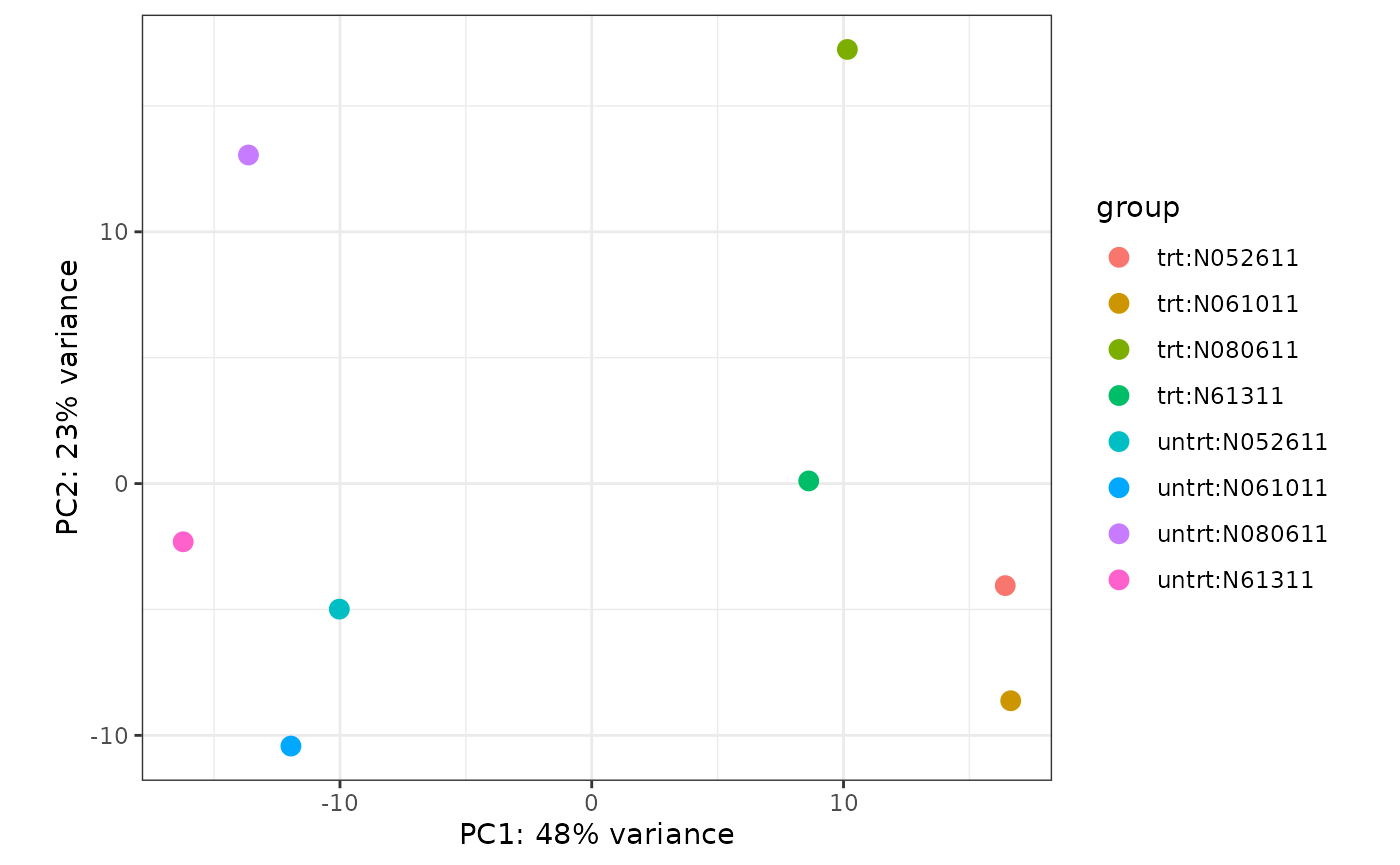
We can embed a javascript-powered interactive scatter plot of the pca result using the viz function. We use the color_aes and shape_aes, we can map the same sample-level covariates to aeshtetics in the plot produced.

viz(pca, color_aes = "dex", shape_aes = "cell")

This uses the normalized counts for the PCA analysis. If we wanted to use the vst transformed data, we could have specified that in the call fcpa() call:

fpca(ddf, assay_name = "vst") %>% 
  viz(color_aes = "dex", shape_aes = "cell")

Removing Batch Effects

When we perform the differential expression analysis, we want to analyze the treatment effects ("dex") while controling for the celltype "cell". The data retrieval functions in the core FacileData package allow for batch correction of normalized data using a simplified wrapper to the limma::removeBatchEffect() function (see ?FacileData::remove_batch_effect).

This functionality is triggered when a covariate(s) is provided in a batch argument, as shown in the code below. Note that we set ntop to 5000, which uses the top 5000 most variable genes for analysis (instead of the default 500). We do this to better perform GSEA on the PCA result afterwards.

cpca <- fpca(ddf, batch = "cell", ntop = 5000)
viz(cpca, dims = 1:3, color_aes = "dex", shape_aes = "cell")

Further interrogation of PCA via GSEA

We can even perform GSEA over any dimension of the PCA result via the ffsea() function (Facile Feature Set Enrichment). This will rank genes by their loadings on the specified PC of interest, then perform a pre-ranked GSEA test (by default, we use limma::cameraPR).

The core of our GSEA functionality is provided by the sparrow package. This includes easy accessor functions for geneset collection retrieval (as a sparrow::GeneSetDb object), as well as delegation of GSEA methods for analysis.

For this, we’ll need a geneset collection stored in a sparrow::GeneSetDb object. We’ll use the MSigDB hallmark genesets for this purpose, and run both "cameraPR" and "fgsea".

gdb <- sparrow::getMSigGeneSetDb(c("H"), "human", "ensembl")
pca.gsea <- ffsea(cpca, gdb, dim = 1, methods = c("cameraPR", "fgsea"))

You can now interactively interrogate the result of the pca.gsea object via the object’s shine() method. This will instantiate a shiny gadget that allows you to browse through its reuslts.

shine(pca.gsea)

And you can visualize the loadings of the genes from a given geneset on the principal component, like so:

viz(pca.gsea, name = "HALLMARK_ADIPOGENESIS")

The GSEA functionality is performed by the sparrow package. Please read that vignette to learn more about its functionality. Also note that performing GSEA on anything but logFC’s or t-statistics (like gene loadings on a principal component) is a newer feature of sparrow, and the visualization needs tweaking (for example, “units” plotted need to be updated (ie. logFC is shown here, but these are not logFC’s).

Differential Expression Analysis

The rnaseqGene workflow tests the differential expression of the dex treatment while controling for the cell identity. The design formula used there was ~ cell + dex, and was set during the call to DESeqDataSet(). We’ll just materialize these results into a data.frame:

dex.dds <- results(dds, contrast=c("dex", "trt", "untrt")) %>% 
  as.data.frame() %>% 
  subset(!is.na(pvalue)) %>% 
  transform(feature_id = rownames(.)) %>% 
  select(feature_id, log2FoldChange, pvalue, padj) %>% 
  arrange(pvalue)
head(dex.dds, 20)

#>                      feature_id log2FoldChange        pvalue          padj
#> ENSG00000152583 ENSG00000152583       4.574919 2.220933e-136 4.003898e-132
#> ENSG00000165995 ENSG00000165995       3.291062 7.839410e-135 7.066444e-131
#> ENSG00000120129 ENSG00000120129       2.947810 3.666925e-130 2.203577e-126
#> ENSG00000101347 ENSG00000101347       3.766995 9.583815e-130 4.319425e-126
#> ENSG00000189221 ENSG00000189221       3.353580 1.098955e-123 3.962392e-120
#> ENSG00000211445 ENSG00000211445       3.730403 4.618318e-112 1.387651e-108
#> ENSG00000157214 ENSG00000157214       1.976773 5.769975e-107 1.486016e-103
#> ENSG00000162614 ENSG00000162614       2.035665 1.323849e-103 2.983294e-100
#> ENSG00000125148 ENSG00000125148       2.210979  2.902397e-97  5.813824e-94
#> ENSG00000154734 ENSG00000154734       2.345604  3.259713e-91  5.876611e-88
#> ENSG00000139132 ENSG00000139132       2.228903  7.578284e-87  1.242012e-83
#> ENSG00000162493 ENSG00000162493       1.891217  8.767337e-87  1.317146e-83
#> ENSG00000134243 ENSG00000134243       2.195712  1.451321e-85  2.012647e-82
#> ENSG00000179094 ENSG00000179094       3.191750  2.120834e-84  2.731028e-81
#> ENSG00000162692 ENSG00000162692      -3.692661  5.646022e-84  6.785765e-81
#> ENSG00000163884 ENSG00000163884       4.459128  2.225442e-80  2.507517e-77
#> ENSG00000178695 ENSG00000178695      -2.528175  6.667027e-79  7.070186e-76
#> ENSG00000198624 ENSG00000198624       2.918436  3.577533e-73  3.583098e-70
#> ENSG00000107562 ENSG00000107562      -1.911670  4.786167e-73  4.541317e-70
#> ENSG00000148848 ENSG00000148848      -1.814543  6.813522e-73  6.141709e-70

On the facile side, we break down the differential expression workflow into two explicit steps. First we define the linear model we will use for testing via the flm_def() function.

To define which samples will be tested against each other, we first specify the covariate used for the sample grouping. The levels of the covariate that specify the samples that belong in the “numerator” of the fold change calculation are specified by the numer parameter. The denom parameter specifies denominator. The batch covarite can be used if there is a covariate we want to control for, like "cell_line" in this case.

xlm <- ddf %>% 
  flm_def(covariate = "dex", 
          numer = "trt", denom = "untrt",
          batch = "cell")
xlm

#> ===========================================================
#> FacileTtestModelDefinition
#> -----------------------------------------------------------
#> Design: ~ 0 + dex + cell
#> Testing contrast over `dex` covariate:
#>   trt - untrt
#> ===========================================================
#>

Now that we have the linear model defined, we can perform a differential expression analysis over it via the fdge() function. Using this funciton, we need to specify:

assay_name: The assay container that holds the assay data we want to perform the test against. The xfds dataset only has one assay ("gene_counts") of type "rnaseq"(assay_info(xfds)), so no need to specify this.
The method to use to perform the analysis. The methods we can use are defined by the type of assay data the assay matrix has. Our "gene_counts" assay is of type "rnaseq". So far, we support the use of the "edgeR-qlf", "voom", and "limma-trend" pipelines for rnaseq analysis (see the output from fdge_methosd("rnaseq")).

There are optional parameters we can specify to tweak the analysis, for instance:

treat_lfc accepts a log2 value which will be used to perform a test against a minimal thershold, using limma’s (or edgeR’s) treat framework.
filter can be used to customize the policy used to remove lowly expressed genes. By default, we wrap the edgeR::filterByExpr() function to produce some sensibly-filtered dataset. Refer to the “Feature Filtering Strategy” section of the ?fdge help page.
use_sample_weights can be set to TRUE if you want to leverage limma’s arrayWeights or voomWithQualityWeights (depending on the method specified).

You can see more details in the ?fdge manual page.

To make our results as comparable to the DESeq results as possible, we will pass the gene identifiers used in the DESeq analysis into the features paramater so we get statistics on those same genes.

We’ll use the the voom framework for our initial analysis:

dex.vm <- fdge(xlm, method = "voom", features = dex.dds$feature_id)

Interpreting the DGE Result

As mentioned previously in the PCA section, every FacileAnalysisResult will provide a tidy() function, which will provide the results of its analysis in tabluar form. In this case, tidy(fdge()) returns a table of the gene-level differential expression statistics, such as the log-fold-change ("logFC"), p-value ("pval"), and the false discovery rate ("FDR").

vm.res <- tidy(dex.vm) %>% 
  arrange(pval) %>% 
  select(feature_id, logFC, t, pval, padj)
head(vm.res, 20)

#> # A tibble: 20 × 5
#>    feature_id      logFC     t     pval     padj
#>    <chr>           <dbl> <dbl>    <dbl>    <dbl>
#>  1 ENSG00000101347  3.77  34.1 2.19e-15 4.33e-11
#>  2 ENSG00000211445  3.71  33.6 2.67e-15 4.33e-11
#>  3 ENSG00000120129  2.93  32.6 4.18e-15 4.33e-11
#>  4 ENSG00000154734  2.31  32.1 5.17e-15 4.33e-11
#>  5 ENSG00000189221  3.31  31.1 8.45e-15 4.77e-11
#>  6 ENSG00000165995  3.27  31.0 8.55e-15 4.77e-11
#>  7 ENSG00000152583  4.55  30.6 1.05e-14 5.04e-11
#>  8 ENSG00000162614  2.02  30.0 1.38e-14 5.78e-11
#>  9 ENSG00000108821 -1.31 -28.5 2.91e-14 1.06e-10
#> 10 ENSG00000157214  1.96  28.2 3.36e-14 1.06e-10
#> 11 ENSG00000134243  2.19  28.2 3.48e-14 1.06e-10
#> 12 ENSG00000107562 -1.95 -27.6 4.74e-14 1.32e-10
#> 13 ENSG00000125148  2.20  27.3 5.59e-14 1.44e-10
#> 14 ENSG00000179593  8.05  25.7 1.32e-13 3.16e-10
#> 15 ENSG00000163884  4.49  24.7 2.35e-13 5.01e-10
#> 16 ENSG00000148175  1.43  24.6 2.40e-13 5.01e-10
#> 17 ENSG00000172403  1.72  24.2 3.07e-13 5.55e-10
#> 18 ENSG00000162692 -3.63 -24.1 3.19e-13 5.55e-10
#> 19 ENSG00000163661  2.24  24.0 3.51e-13 5.55e-10
#> 20 ENSG00000178695 -2.52 -24.0 3.53e-13 5.55e-10

Deep Interaction via shine()

The shine() function over an fdge() result presents the user with the table of gene-level differential expression statistics, which is linked to a view over the expression of the gene of interest over the given contrast.

Since "cell_line" was used as a batch term in the linear model, the sample-level expression values plotted (by default) are batch-corrected. You can toggle batch correction off to see the effect it has on the data.

shine(dex.vm)

You can visualize and interact with a volcano plot as well. Drawing the volcano plot is initially disabled, however, since it currently creates an interactive scatter plot view over all of the (potentially thousands) genes analyzed. This can overwhelm CPUs with lower end GPUs.

Embeddable interactive graphics via viz()

The viz() function on an fdge() result can be used to make a volcano plot, MA plot, or to show the expression profiles of a set of genes across the groups that were tested.

We can view what the differential expression of the top result looks like, with and without batch corrected values.

viz(dex.vm, features = head(vm.res, 1))

In the same way that you can disable plotting the batch-corrected expression values per sample in the shiny gadget, you can also turn it off here, as well:

viz(dex.vm, features = head(vm.res, 1), batch_correct = FALSE)

This is how you can query the FacileDataSet directly to retrieve these expression values and plot them manually.

dat.bc <- dex.vm %>% 
  samples() %>% 
  fetch_assay_data(features = head(vm.res, 1),
                   assay_name = "vst",
                   batch = "cell") %>% 
  with_sample_covariates("dex") %>% 
  mutate(type = "batch_corrected")
dat.o <- dex.vm %>% 
  samples() %>% 
  fetch_assay_data(features = head(vm.res, 1), normalized = TRUE) %>% 
  with_sample_covariates("dex") %>% 
  mutate(type = "original")

dat <- bind_rows(dat.bc, dat.o)
ggplot(dat, aes(x = dex, y = value)) +
  geom_boxplot(outliser.shape = NA) +
  geom_jitter(aes(color = dex), width = 0.2) +
  facet_wrap(~ type)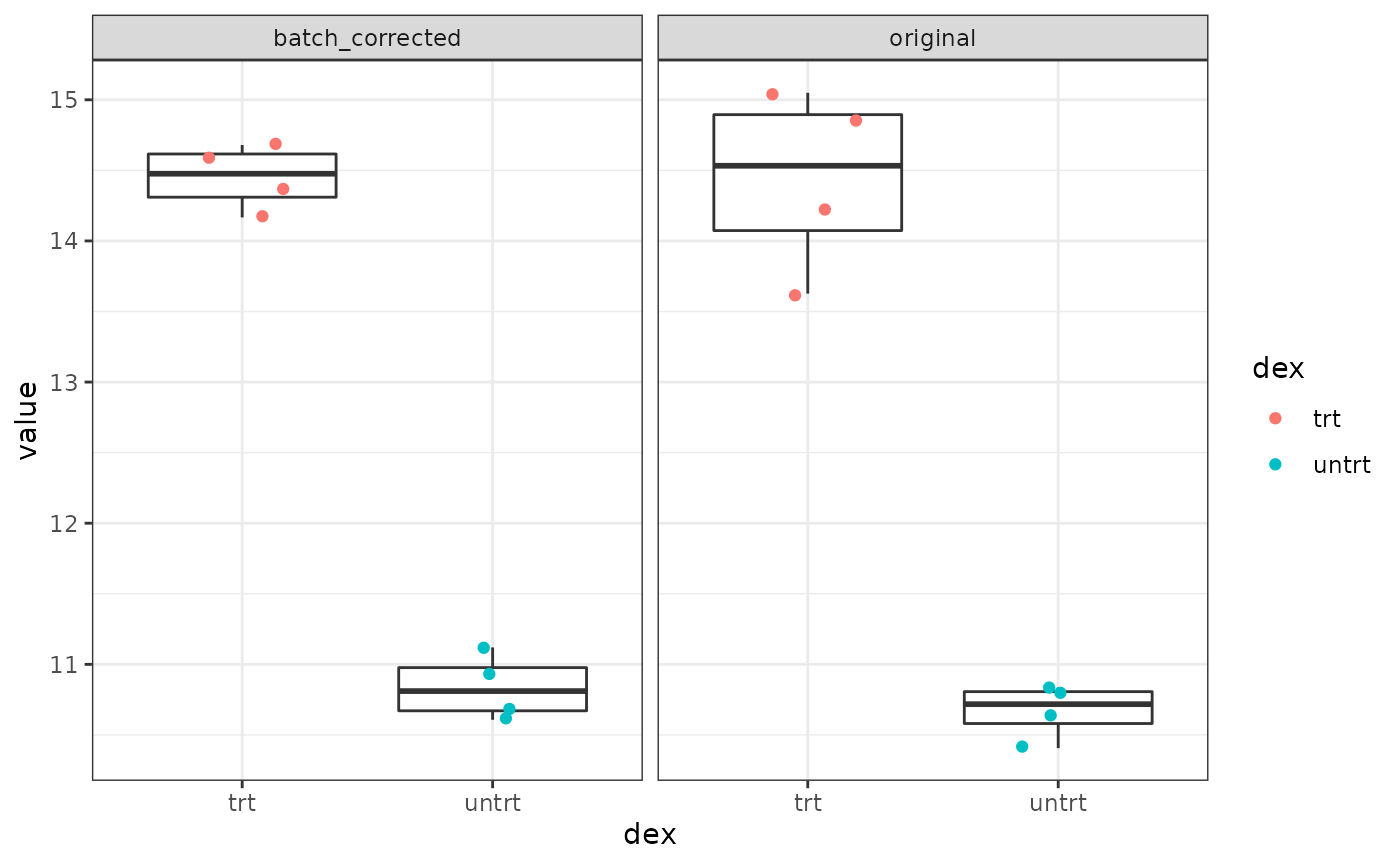

We can also visualize the differential expresion result as a volcano plot, and highlight which of the genes were also in DESeq2’s top 50 results. By default, these plots use webgl, but we still restrict it to only show the top 1500 genes in the volcano. You can set this to Inf to show all of them.

viz(dex.vm, type = "volcano", ntop = 1500,
    highlight = head(dex.dds$feature_id, 50))

… or an MA plot …

# Instead of taking the top 1500, which leaves a solid empty space in the
# 'low-signicance zone', like the volcano above, we can pick a random set of
# 15000 genes, then highlight the top ones from the DESeq2 result.
# You an try the same trick with the volcano plot above.
viz(dex.vm, type = "ma", 
    # ntop = 1500,
    features = features(dex.vm) %>% sample_n(1500),
    highlight = head(dex.dds$feature_id, 50))

Embeddable interactive summaries via report()

FacileAnalysisResult objects also provide report() functions. Their goal is to weave together a number of views and statistics from an analysis that are most presented together when we attempt to share analytic results with collaborators within an Rmarkdown document.

For instance, when reporting a differential expression analysis result, it is often convenient to supply a table of signficant results combined with something like a volcano plot.

The report() function over a FacileTtestAnalysisResult will plot the volcano of the ntop genes, and uses the crosstalk package to link this to a linked table of gene-level statistics. The individual genes provide link-outs to their information page on the ensembl website.

report(
  dex.vm, ntop = 500,
  caption = paste(
    "Top 500 results from a differential expression analysis of the airway",
    "dataset treated and control samples, adjusting for the `cell_line`",
    "effect"))

Differential Expression Results
Top 500 [FDR 0.10, abs(logFC) >= 1.00]

Design: ~ 0 + dex + cell

Tested: dex: trt - untrt

Top 500 results from a differential expression analysis of the airway dataset treated and control samples, adjusting for the `cell_line` effect

Using the edgeR quasi-likelihood framework

We have tested our contrast of interest using the limma/voom statistical framework (fdge(xlm, method = "voom")), but you might want to use a different framework.

Currently the following options are supported to test rnaseq-like data:

fdge_methods("rnaseq")

#>   assay_type  dge_method bioc_class default_filter robust_fit robust_ebayes
#> 1     rnaseq        voom    DGEList           TRUE      FALSE         FALSE
#> 2     rnaseq   edgeR-qlf    DGEList           TRUE       TRUE         FALSE
#> 3     rnaseq limma-trend    DGEList           TRUE      FALSE         FALSE
#>   trend_ebayes can_sample_weight
#> 1        FALSE              TRUE
#> 2        FALSE             FALSE
#> 3         TRUE              TRUE

You can swap out "voom" for any of the methods listed there. Let’s use the edgeR quasi-likelihood framework, instead:

dex.qlf <- fdge(xlm, method = "edgeR-qlf", features = dex.dds$feature_id)

Did the fdge() analysis work?

Now that we’ve looked at some ways to interact with our results, and tweak the way in which they were run, it would be nice to know if the simplified interface presented in the facile ecosystem runs analyses that produces accurate and comparable results.

We can check to see how concordant the statistics generated by the "voom" and "edgeR-qlf" methods produced via fdge() are when compared to the DESeq2 result. We’ll join the results of all three analysis together to see.

cmp <- tidy(dex.vm) %>% 
  select(feature_id, symbol, logFC.vm = logFC, pval.vm = pval) %>% 
  inner_join(dex.dds, by = "feature_id") %>% 
  inner_join(
    select(tidy(dex.qlf), feature_id, logFC.qlf = logFC, pval.qlf = pval),
    by = "feature_id") %>% 
  mutate(qlf.pval = -log10(pval.qlf), 
         vm.pval = -log10(pval.vm),
         d2.pval = -log10(pvalue))

cmp %>% 
  select(qlf.pval, vm.pval, d2.pval) %>% 
  pairs(main = "-log10(pvalue) comparison", pch = 16, col = "#3f3f3f33")

cmp %>% 
  select(qlf.logFC = logFC.qlf,
         vm.logFC = logFC.vm,
         d2.logFC = log2FoldChange) %>% 
  pairs(main = "logFC comparison", pch = 16, col = "#3f3f3f33")

The test-fdge.R unit tests ensures that the results produced via the facile flm_def() %>% fdge() pipeline are the same as the ones produced using their corresponding standard bioconductor maneuvers over the same data.

Gene Set Enrichment Analysis

As is the case in the PCA -> GSEA analysis performed above, GSEA here is performed downstream of the differential expression result. We need to specify the geneset collection to use for GSEA, as well as the GSEA methods we want to perform.

dge.gsea <- ffsea(dex.vm, gdb, methods = c("ora", "cameraPR"))

Calling shine(dge.gsea) on this GSEA result will pull up a shiny gadget that allows you to interactively explore the signifcant GSEA results from from this differential expression analysis.

shine(dge.gsea)

The shiny gadget will look similar to the one produced by running ffsea() on the fpca() result, depicted above. The screen capture is not included in this vignette to save (HD) space.

Side Loading Data (for svaseq)

The rnaseqGene workflow then outlines how one could use sva::svaseq to adjust for unknown batch effects.

library(sva)
dat  <- counts(dds, normalized = TRUE)
idx  <- rowMeans(dat) > 1
dat  <- dat[idx, ]
mod  <- model.matrix(~ dex, colData(dds))
mod0 <- model.matrix(~ 1, colData(dds))
deseq.sva <- svaseq(dat, mod, mod0, n.sv = 2)

#> Number of significant surrogate variables is:  2 
#> Iteration (out of 5 ):1  2  3  4  5

Although svaseq isn’t directly supported in the facile workflow, we can still do this by first extracting the data we need into objects that svaseq can use, then marrying the surrogate variables that were estimated over our samples back with the FacileDataSet for use within the differential expression analysis workflow.

To extract the data from the FacileDataSet to initially run svaseq, we will:

Extract the counts used from the genes/samples in our differential expression analysis; and
Create a data.frame that can be used with the model.matrix calls above.

We can get all of the normalized count data from the expression container with the following call:

norm.dat <- fetch_assay_data(ddf, as.matrix = TRUE, normalized = TRUE)

This will use the stored library size and normalization factors within the FacileDataSet to retrieve all of the the log2(cpm) data from these samples.

We can do a bit better, though, in the sense that we can use the data normalized in the same way as it was for the differential expression analysis. We can ask a FacileAnalysisResult, like dex.qlf, what samples it was run on using the samples() function:

samples(dex.qlf) %>% head()

#> # A tibble: 6 × 6
#>   dataset sample_id  cell    dex   lib.size norm.factors
#>   <chr>   <chr>      <fct>   <fct>    <dbl>        <dbl>
#> 1 dataset SRR1039508 N61311  untrt 20637971        1.06 
#> 2 dataset SRR1039509 N61311  trt   18809481        1.03 
#> 3 dataset SRR1039512 N052611 untrt 25348649        0.983
#> 4 dataset SRR1039513 N052611 trt   15163415        0.949
#> 5 dataset SRR1039516 N080611 untrt 24448408        1.03 
#> 6 dataset SRR1039517 N080611 trt   30818215        0.973

You’ll see what get a few other useful things, too:

The cell and dex covariates are added to the samples, because they were used within the flm_def() -> fdge() pipeline we ran.
The lib.size and norm.factors columns were added from the DGEList that was ultimately materialized and used within the call to fdge(). These were recalculated “fresh” after we filtered down to the genes that were specified via the fdge(..., filter) parameter.

Let’s get our normalized expression data now:

fcounts <- dex.qlf %>% 
  samples() %>% 
  fetch_assay_data(features = rownames(dat), 
                   assay_name = "counts", normalized = TRUE, log = FALSE,
                   as.matrix = TRUE)

These data will be returned in the same (column) order as is specified in the samples(dex.qlf) data.frame:

stopifnot(
  all.equal(sub("dataset__", "", colnames(fcounts)), colnames(dat)),
  all.equal(rownames(fcounts), rownames(dat)),
  # let's check only some values to make it quick
  all.equal(fcounts[1:100,], dat[1:100,], check.attributes = FALSE))

Now we have the pieces we need to run svaseq over our facile data:

fmod  <- model.matrix(~ dex, samples(dex.qlf))
fmod0 <- model.matrix(~ 1, samples(dex.qlf))
facile.sva <- svaseq(fcounts, fmod, fmod0, n.sv = 2)

#> Number of significant surrogate variables is:  2 
#> Iteration (out of 5 ):1  2  3  4  5

As expected, the surrogate values calculated from both datasets are the same, but it never hurts to check:

par(mfrow=c(1,2))
plot(deseq.sva$sv[, 1], facile.sva$sv[, 1], pch = 16,
     main = "SV1", xlab = "Original", ylab = "Facile")
abline(0, 1, col = "red")
plot(deseq.sva$sv[, 2], facile.sva$sv[, 2], pch = 16,
     main = "SV2", xlab = "Original", ylab = "Facile")
abline(0, 1, col = "red")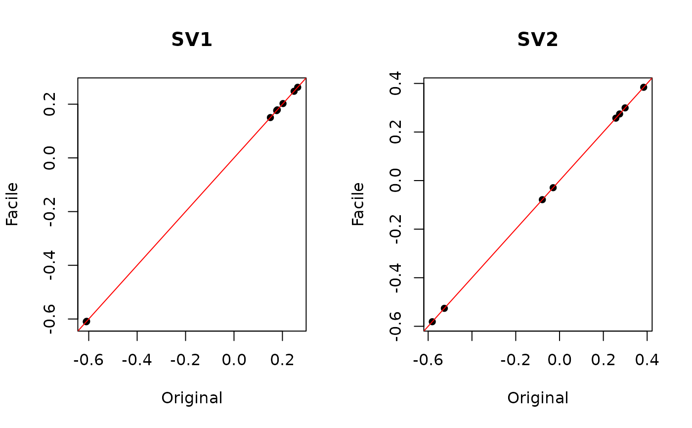

Now we add these to our samples facile_frame and redo the linear model and perform differential expression analysis using only the surrogate variables to contorl for batch (as is done in the rnaseqGene workflow).

sva.qlf <- samples(dex.qlf) %>% 
  mutate(SV1 = facile.sva$sv[, 1], SV2 = facile.sva$sv[, 2]) %>% 
  flm_def(covariate = "dex", 
          numer = "trt", denom = "untrt",
          batch = c("SV1", "SV2")) %>% 
  fdge(method = "edgeR-qlf", features = features(dex.qlf))

How do these compare with the original quasilikelihood analysis?

cmp.qlf <- tidy(dex.qlf) %>% 
  select(feature_id, symbol, logFC, pval) %>% 
  inner_join(
    select(tidy(sva.qlf), feature_id, logFC, pval),
    by = "feature_id")

ggplot(cmp.qlf, aes(x = logFC.x, y = logFC.y)) +
  geom_point(alpha = 0.8) +
  geom_abline(intercept = 0, slope = 1, color = "red") +
  xlab("logFC original") +
  ylab("logFC with sva") +
  ggtitle("logFC comparison with cell_line batch vs svaseq batch")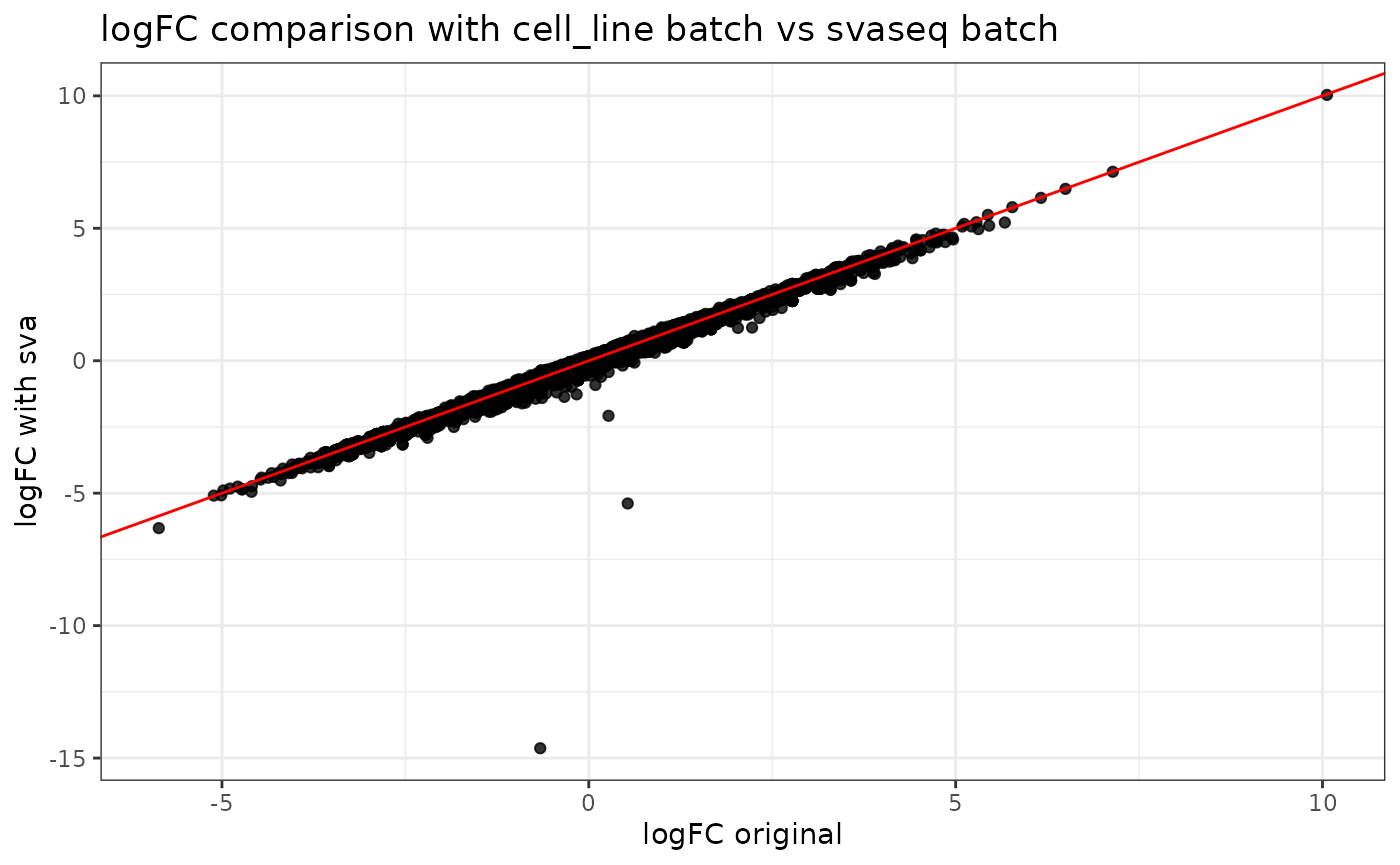

ggplot(cmp.qlf, aes(x = -log10(pval.x), y = -log10(pval.y))) +
  geom_point(alpha = 0.8) +
  geom_abline(intercept = 0, slope = 1, color = "red") +
  xlab("-log10(pvalue) original") +
  ylab("-log10(pvalue) with sva") +
  ggtitle("pvalue comparison with and without svaseq")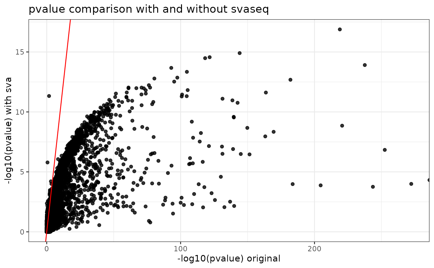

Visualizing effects of batch correction

We’ve tested two different methods of batch correction in this analysis workflow. The first was to explicitly select "cell_line" as a batch effect. The second was to use svaseq to identify unknown sources of variance we can correct for.

Let’s see how these effect the expression levels of a gene of interest.

batches <- list(
  none = NULL,
  cell_line = "cell",
  SV1 = "SV1",
  SVboth = c("SV1", "SV2"))
dat <- lapply(names(batches), function(bname) {
  samples(sva.qlf) %>% 
    with_assay_data("ENSG00000101347", batch = batches[[bname]], log = TRUE) %>% 
    mutate(group = bname)
})
dat <- bind_rows(dat)

ggplot(dat, aes(x = dex, y = ENSG00000101347)) +
  geom_boxplot(outlier.shape = NA) +
  geom_jitter(aes(color = cell), width = 0.25) +
  facet_wrap(~ group)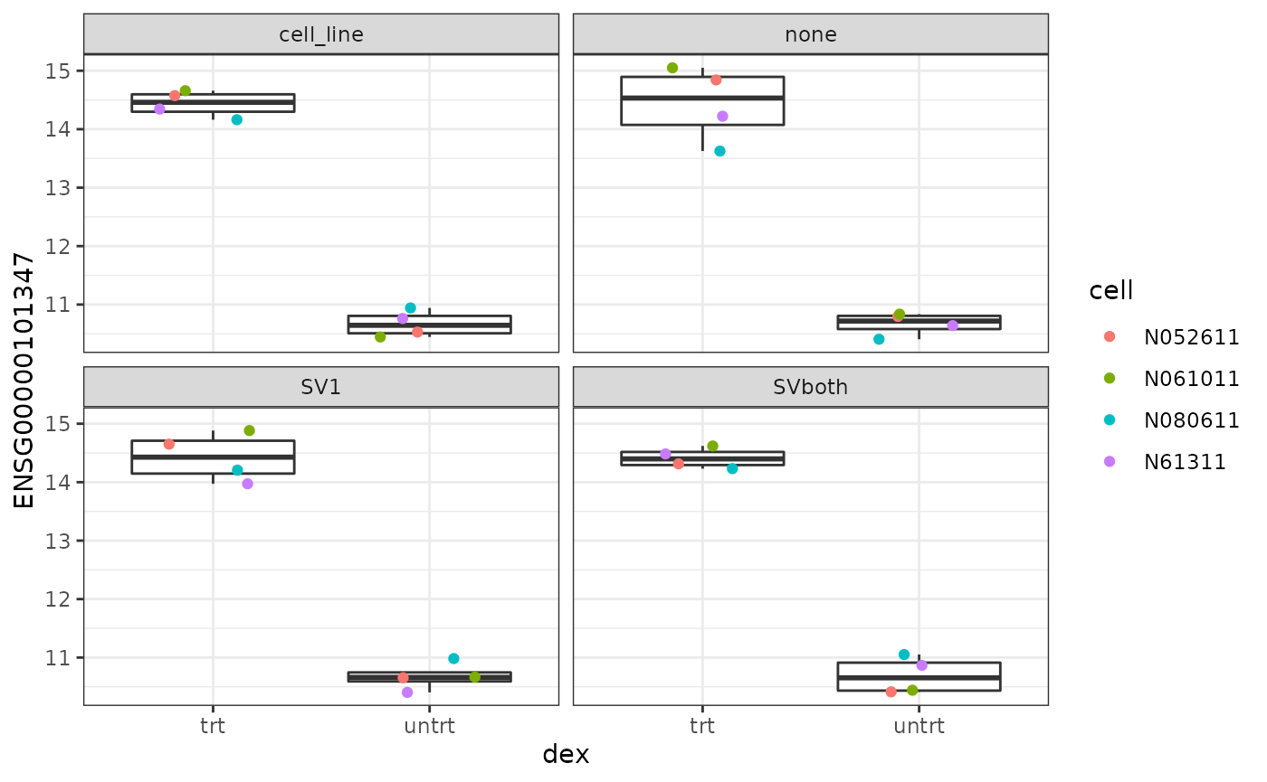

facile_frame objects override dplyr-verbs, so most dplyr-based data manipulations ensure that the facile_frame that is returned maintains its connection to its FacileDataStore. Unfotunately, we don’t provide a facile-version of the bind_rows function, since it dplyr::bind_rows() isn’t an S3 generic because its first argument is .... We’ll provide a workaround to this in due time.

GUI Driven Analysis

The analyses defined in this package should be equally available to coders, as well as those who aren’t proficient in code (yet) but want to query and explore these data.

Gadget-ized versions of these analyses are available within this package that can be invoked from within an R workspace. The same modules used in the gadgets can also be weaved together in a standalone shiny app, that can be completely driven interactively.

FacileAnalysis Gadgets

The same differential expression analysis we performed in code, like so:

dex.qlf <- ddf %>% 
  flm_def(covariate = "dex", 
          numer = "trt", denom = "untrt",
          batch = "cell") %>% 
  fdge(method = "edgeR-qlf")

can also be done using the fdgeGadget(). Shiny modules for the flm_def and fdge functions are chained together so that they can be configured as above, and the results of the interactive, gadget-driven analysis below will be the same as the one produced above.

dex.qlf2 <- fdgeGadget(ddf)

Once the user closes the gadget (hits “OK”), the result will be captured in dex.qlf2. You can then tidy() it to get the differential expression statistics as before, or use this as input to ffsea() for feature set enrichment analysis, either via code, or via a gadget.

The second call in the code below launches a shiny gadget to perform a GSEA. It will return a result that is identical to the first.

dex.gsea2 <- ffsea(dex.vm2, gdb, method = c("ora", "cameraPR"))
dex.gsea3 <- ffseaGadget(dex.vm2, gdb)

Try it!

Closing Thoughts

We’ve covered a bit of ground. Here are some things to keep in mind.

Extracting a facile_frame from a FacileDataSet should be the starting point for most analyses. Tidy-like functions are defined over a facile_frame that allow the user to decorated it with more data whenever desired. The (fetch|with)_assay_data() and (fetch|with)_sample_covariates() functions are your gateway to all of your data.
FacileAnalysisResult objects provide a number of methods that enable the analyst to interrogate it in order to understand it better.
- shine() provides a rich, shiny-powered view over the result.
- viz() provides will provide a variety of JS-powered views over the data.
- report() will wrap up a number of useful views over a result and dump them into an Rmarkdown report, with some level of JS-based interactivety.
- We briefly mentioned signature() and ranks(), but don’t talk about why they are here. Briefly, analyses usually induce some ranking over the features that they were performed over. Like a differential expression result produces a ranking over its features (genes). We think that these are useful general concepts that analysts would want to perform over analyses of all types, and defining them will help to make analyses more fluid / pipeable from one result into the next. More on that later.
Analyses within this package can (should) be able to be conducted equally using code, a GUI, or a hybrid of the two.

This is still a work in progress. Not every analysis type is developed to the same level of maturity. For instance:

report() isn’t implented for ffsea() and fpca() objects
shine(fpca()) is functional, but still needs some more work.

… and you’ll find some other wires to trip over. Please file bug reports when you do!

Steve Lianoglou

5/17/2019

Overview

Setup

Data Preparation

Prepare the DESeqDataSet

Enable use of DESeqDataSet via the Facile API

Principal Components Analysis

Interrogating a PCA Result

Just show me the numbers with tidy()

Deep Interaction via shine()

Embeddable interactive graphics with viz()

Removing Batch Effects

Further interrogation of PCA via GSEA

Differential Expression Analysis

Interpreting the DGE Result

Deep Interaction via shine()

Embeddable interactive graphics via viz()

Embeddable interactive summaries via report()

Using the edgeR quasi-likelihood framework

Did the fdge() analysis work?

Gene Set Enrichment Analysis

Side Loading Data (for svaseq)

Visualizing effects of batch correction

GUI Driven Analysis

FacileAnalysis Gadgets

Closing Thoughts