Overview
The FacileData package was written to facilitate easier analysis of large, multi-assay, high-throughput genomics datasets. To this end, the FacileData package provides two things:
- A FacileData Access API that defines a fluent interface over multi-assay genomics datasets that fits into the tidyverse. This enables analysts to more naturally query and retrieve data for general exploratory data analysis; and
- A reference implementation of a datastore that implements the FacileData Access API called a FacileDataSet. The
FacileDataSetprovides efficient storage and retrieval of arbitrarily large high-throughput genomics datasets. For example, a singleFacileDataSetcan be used to store all of the RNA-seq, microarray, RPPA, etc. data from the The Cancer Genome Atlas. This singularFacileDataSetallows analysts easy access to arbitrary subsets of these data without having to load all of it into memory.
Background
The Bioconductor ecosystem provides a number of data containers, like the SummarizedExperiment to store high-throughput genomics data and the metadata that goes along with it. These containers provide a consistent way for users to access the different aspects of the data that are required to successfully analyze genomics data and have served the community well for a long time, especially in the context of single-experiment projects.
Storing data in these containers, however, is sub-optimal in a few situations:
- When the analyst wants to perform more general exploratory data analysis techniques over the data (like simple scatterplots, boxplots, etc.). When the analyst is contrained by the data access API defined by a SummarizedExperiment, creating simple scatter and boxplots (for exmaple) can become quite tedious; and
- When the analyst is analyzing similar data over very large datasets, such as the entirety of the data from The Cancer Genome Atlas (TCGA), particularly due to the fact that these data containers want to store all of the data in RAM.
The fluent and efficient analysis of data from the TCGA poses even more problems since a multitude of assays have been run over each sample, such as RNA-seq, microarrays, exome-seq, etc. With all of this data in hand, analysts may want to look at how gene expression compares to copy number, or miRNA expression, etc.
In these scenarios, a single SummarizedExperiment is no longer up to the task of storing these data since the “feature-space” (rows of the SummarizedExperiment) of all the assays within a singular SummarizedExperiment must be equal.
These problems manifest themselves when we consider even the simplest of analysis scenarios, such as processing an RNA-seq assay into two different feature spaces, (1) gene-level counts; and (2) transcript-level counts. One would have to create two separate SummarizedExperiments with the same columns and colData, but different assay matrices given the different feature-spaces (genes vs. transcripts).
Using a single FacileDataSet, all of these data can be stored in the same data container, and the FacileData API allows analysts to retrieve data from each effortlessly.
Recently, the Bioconductor community has developed the MultiAssayExperiment objet to address many of the same issues the FacileDataSet was built to address. We can consider these complementary efforts, for now. One can imagine using a MultiAssayExperiment as a backend to store these data, and create a thin FacileData API wrapper, to create a FacileMultiAssayExperiment.
FacileData API
The FacileData API defines a set of query and retrieval functions over multi-assay genomics datasets that fits into the tidyverse.
To provide illustrative examples of the utility of the FacileData API, we rely on the FacileTCGADataSet package, which provides the full RNA-seq expression, miRNA expresion, and copy number data across all 33 indications (11,000+ samples) from the TCGA. Please see the FacileTCGADataSet package for more information regarding how these data were put together, and how to extend it.
As a teaser, we provide code snippets that show how to plot HER2 copy number vs. expression across the TCGA “BLCA” and “BRCA” indications using the FacileDataSet. We’ll then compare that to how the same code might be written using more traditional bioconductor containers.
library(FacileData)
# library(FacileTCGADataSet)
library(ggplot2)
# tcga <- FacileTCGADataSet()
tcga <- exampleFacileDataSet()

samples <- filter_samples(tcga, indication %in% c("BLCA", "BRCA"))
features <- filter_features(tcga, name == "ERBB2")

fdat <- samples %>%
  with_assay_data(features, assay_name = "rnaseq", normalized = TRUE) %>%
  with_assay_data(features, assay_name = "cnv_score") %>%
  with_sample_covariates(c("indication", "sex"))

ggplot(fdat, aes(cnv_score_ERBB2, ERBB2, color=sex)) +
  geom_point() +
  facet_wrap(~ indication)
Example Analysis
library(FacileData)
library(dplyr)
# library(FacileTCGADataSet)
# tcga <- FacileTCGADataSet()
tcga <- exampleFacileDataSet()
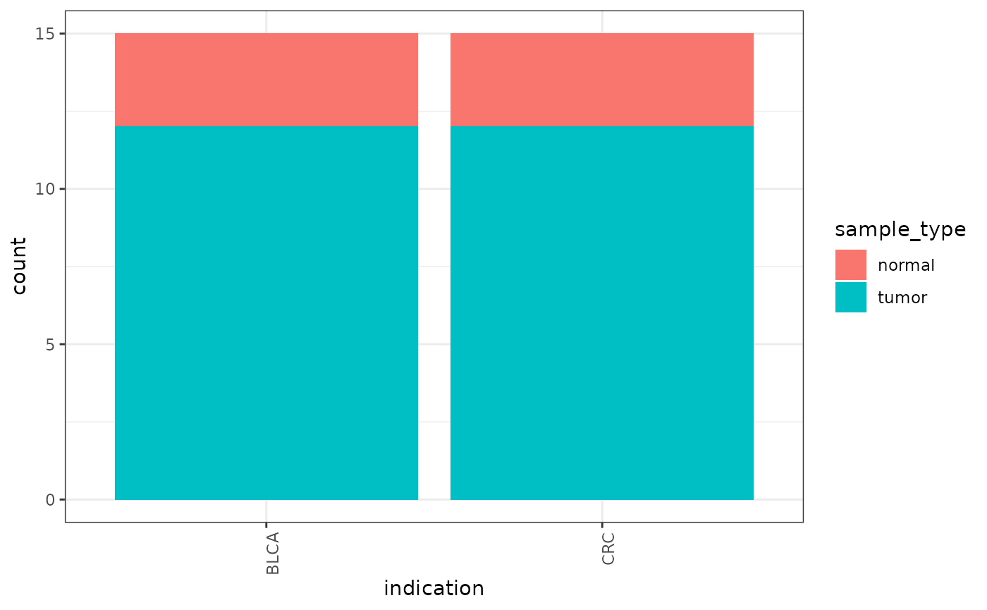
distro <- samples(tcga) %>%
  with_sample_covariates(c("indication", "sample_type"))
ggplot(distro, aes(indication, fill=sample_type)) +
  geom_bar() +
  theme(axis.text.x=element_text(angle=90, hjust=1))
FacileData Access API
The base interface is the FacileDataStore. There are no objects of this class, it rather serves as an interface that should be implemented by a subclass, i.e. a FacileDataSet, or a FacileSummarizedExperiment. An object that is(x, "FacileDataStore") == TRUE is assumed to implement the entire FacileData API.
Broadly speaking, there are two classes of functions that are used to pull data out of a FacileDataSet, the fetch_* and with_* functions. To a first approximation, we can consider the fetch_* functions to be the lowest level functions, and the with_* functions are higher-level accessors.
The with_* functions were written so that they can naturally be combined in pipe (%>%) data-manipulation chains. They provide analysts with a fluent and succinct API with which to perform exploratory data analyses.
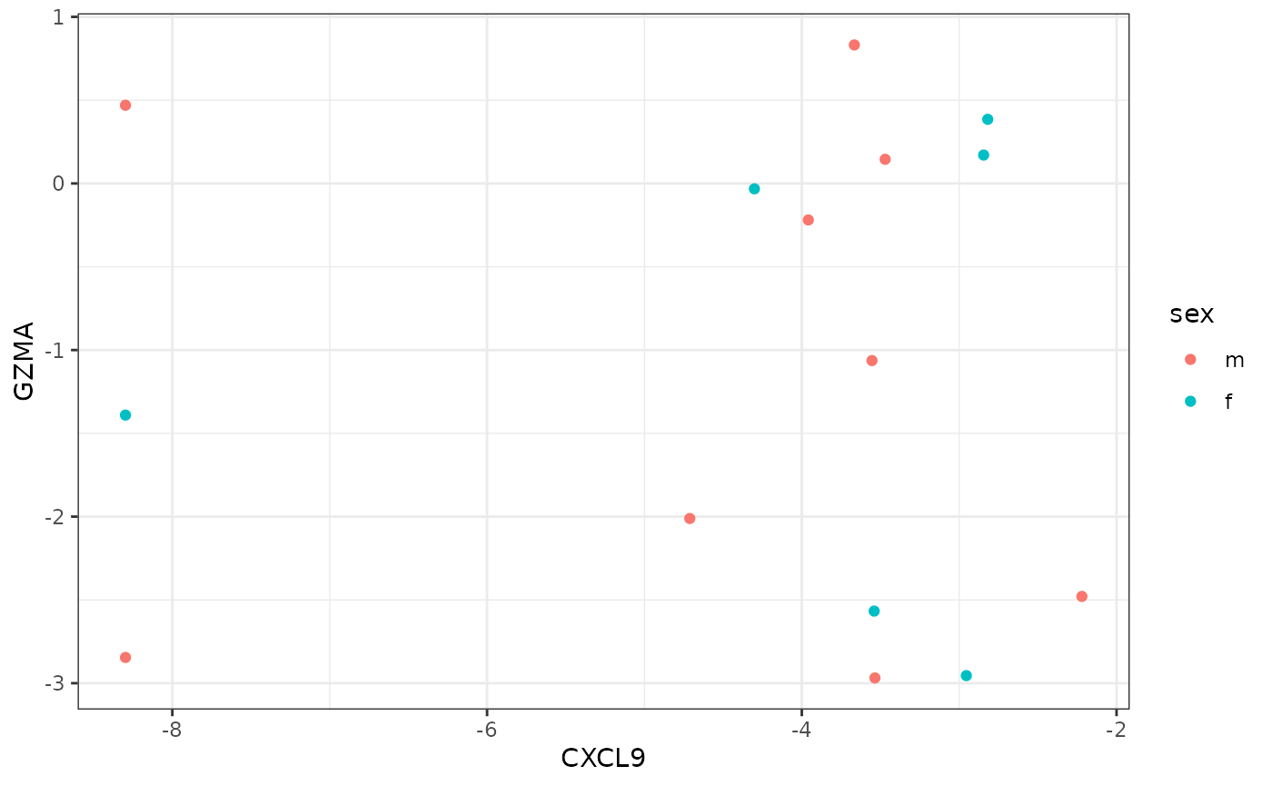
For example, to retrieve normalized RNA-seq expression values for CXCL9 and GZMA along with survival and sex information for the samples inin the TCGA bladder (“BLCA”) indication, you can write:
features <- filter_features(tcga, name %in% c("CXCL9", "GZMA"))

blca.dat <- tcga %>%
  filter_samples(indication == "BLCA") %>%
  with_assay_data(features, assay_name="rnaseq") %>%
  with_sample_covariates(c("OS", "sex"))

ggplot(blca.dat, aes(CXCL9, GZMA, color=sex)) +
  geom_point()
Function list
Currently the API consists of:
- filter_features
- filter_samples
- fetch_assay_data
- with_assay_data
- fetch_assay_score (x): just use
fetch_assay_data(..., aggregate = TRUE) - fetch_custom_sample_covariates (this probably isn’t user facing)
- fetch_sample_covariates
- with_sample_covariates
- fetch_sample_statistics (x)
- fetch_samples (x)
Functions marked with (x) indicate that this function should be on its way out.
Please see the manpages for these functions for more details.
Classes
-
facile_frame: this works like atibble, but has a handle to theFacileDataStorethat it came from in a slot. We provide.facet_frameimplementations for the dplyr andbase::subsetlike verbs, as well as[and[[so that we can manipulate this as transparently as possible.
MultiAssayExperiment API Comparsion
Since MAE’s are the closest thing to a datastore that should also easily accomodate the FacileData API, we’d like to compare how similar analyses are done between the two approaches.
Let’s collect MAE use cases in the wild here, and compare ease of data retreival and analysis using between the two.
- Mini TCGA analysis with MAE from the [Management of genome-scale data section][ph525mae] of the PH525x Biomedical Data Science book by Love et al.